Redistricting Reform

Now that we have assessed gerrymandering’s growing threat, let us move on to the business of solving it, or at least mitigating its worst effects. This section provides an overview of the current redistricting reform landscape, including a taxonomy of redistricting commissions based on composition, authority, and charges. It also frames three central questions for thinking about redistricting (or anti-gerrymandering) reform:

1. What makes a district map “fair”?
2. Can redistricting commissions make maps fairer?
3. Are there meaningful differences in types of redistricting commissions?

What makes a district map “fair”?

Fairness is a contested concept. Much of contemporary political theory is devoted to questions of fairness. Though primarily these debates involve the fair distribution of resources, they show how difficult it is to agree on a baseline. Moreover, fairness typically requires trading off among competing values, none of which can be maximized.

Nonetheless, if perfect fairness is impossible to define, there are degrees of fairness. It may be a continuum in which the ends are fuzzy and uncertain, but it is also possible to make comparisons between more or less fair.

Can redistricting commissions make maps fairer?

If we view fairness not as an absolute, but as a continuum, it becomes possible to assess the performance of redistricting commissions along a scale. However, because the ends of the fairness continuum are fuzzy and contested, there are limits to how fair maps can be. Still, in general, across a range of dimensions, redistricting commissions can make maps fairer.

Are there meaningful differences in types of redistricting commissions?

There are variations in types of commissions. In general, the more independent commissions are from state legislatures, the better they perform on a range of fairness metrics.

To dive more deeply into these questions, this report will now address in more detail the particular ways in which we evaluate districts, the challenges of measuring each of the five main standards—partisan neutrality, competitiveness, compactness, keeping communities of interest together, and fair minority representation—and the ways in which these standards are often at odds with each other.

We all think we know what partisan gerrymandering is. It is the process by which partisans draw legislative districts to ensure that their party wins as many districts as possible, given the underlying distribution and partisan proclivities of voters.

So, for example, numerous studies have found that the 2011 redistricting gave Republicans a disproportionate advantage in Congress. Notably, in the 2012 elections, Republicans won more seats (53.8 percent) than Democrats (46.2 percent) in the House, despite earning a smaller share of the popular vote (46.9 percent) than Democrats (48.3 percent).¹ This appears to be a clear bias in favor of Republicans. At the state level, biases in favor of one party over the other are even more extreme.²

But what is the alternative—partisan neutrality? Intuitively, it is a simple principle: parties should win seats in proportion to how many votes they get. So, if a party gets 60 percent of the votes statewide, it should get no more or less than 60 percent of the seats statewide. However, this intuitive understanding of partisan neutrality is at odds with the way in which the current system of districting operates. Understanding how the number of seats per district (which political scientists call “district magnitude”), and the distribution of partisan support impact the possibilities for partisan neutrality is crucial for understanding the challenges that both independent redistricting commissions and courts face in deciding what is fair within the single-member district context.

Measuring Partisan Neutrality

How should we measure partisan neutrality in districting?

Unfortunately, there is no clear answer. As one recent review of 18 different measures observes, “Unfortunately, there is no consensus as to which of these measures works the best.”³ This lack of a consensus standard helped provide an excuse for the Supreme Court to say that this issue was not justiciable in Rucho v. Common Cause.

Here we will conduct a brief review of several measures, including proportionality, symmetry, efficiency, and improbability and intent. There are a few reasons to spend some time on the complications of these measures. The first, and most important reason, is to appreciate that there is no perfect standard of partisan neutrality, though there are plenty of decent measures.

It is not hard to determine when a districting map is blatantly unfair. Under those cases, any measure, or an aggregate of measures will work. But in an era in which elections are often decided narrowly, “fairness” can depend on which measure one prefers. And if some measures point one way, and some measures point the other way, both sides can find reasons to feel like they were cheated. To a large extent, fairness will always be in the eye of the (partisan) beholder.

Again, we will get into the weeds on measuring fairness here. Though this may seem like an academic discussion (it partly is), the details matter. They help us to understand how difficult it is to draw truly “fair” maps. The difficulties in declaring true partisan neutrality follow from two well-known peculiarities of single-member districts:⁴

1. The “winner’s bonus” (a.k.a. “loser’s penalty”). Under single-member districts, a party that gets a majority of votes typically gets a bonus share of seats in excess of pure proportionality.
2. The importance of geography. Under single-member districts, where voters live is more important than how many voters support each party. This peculiar property is what makes gerrymandering such a dangerous weapon. But it also accounts for a fair degree of “natural gerrymandering” that can undermine partisan neutrality as well. In short, Democrats waste a lot of votes in lopsided urban districts, begging the question of whether or not a fair map should correct for this.

Attempts to make maps fair are also complicated by other normative values of districting: compactness, keeping communities of interest together, competitiveness, and adequate minority representation through majority-minority districts.

Different measures of fairness attempt to account for these complications differently, based on different conceptions of what would be perfectly fair.

To be sure, all of these measures are highly correlated, though some are more closely correlated than others.⁵ However, different measures applied to the same maps can consider the same maps to be tilted in favor of Republicans or in favor of Democrats.

Proportionality

The most simple standard, of course, is proportionality. That is, the share of a party’s seats should match its share of votes. However, it is a well-known and long-described property of single-member districts that they do not produce proportional results at a national level.⁶

One way to see this is to look at the modern history of U.S. House elections.

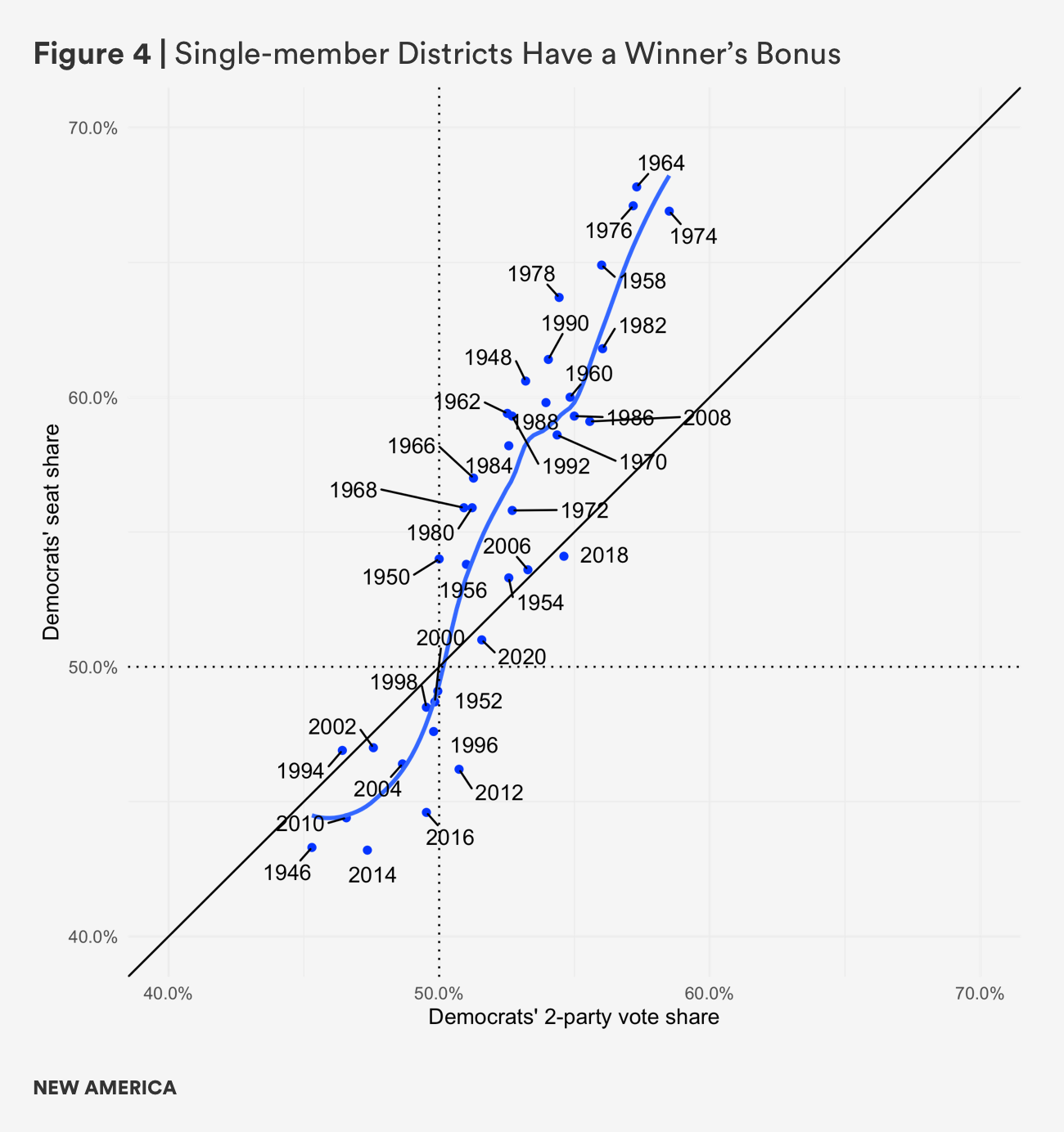
As we can see, the seats-to-vote ratio has a winner’s bonus. In the years in which Democrats captured the majority of votes, they tended to get even a larger percentage of the seats. The blue line is a smoothed curve tracing the relationship between seats and votes across all elections. The black line is perfect proportionality.

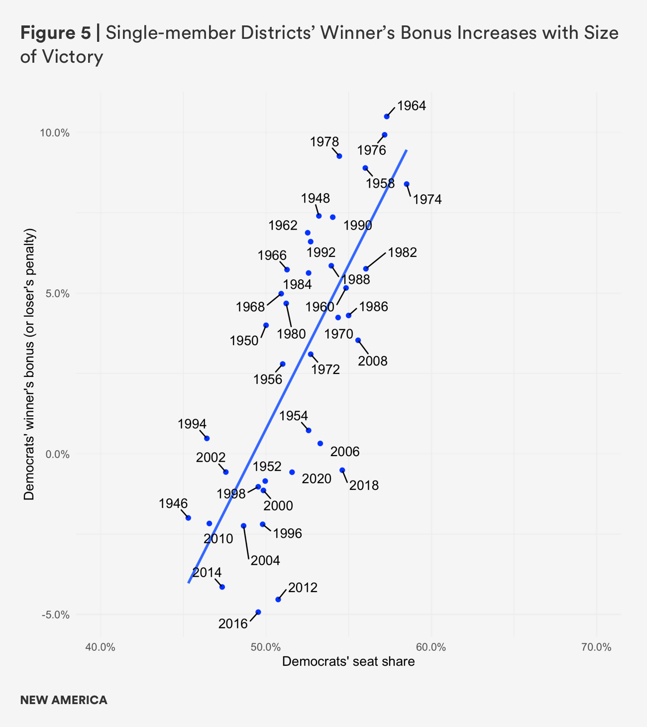
Another way to see this is to look at the relationship between Democrats’ seat share and the size of the winner’s bonus, which increases pretty much linearly as Democrats win a larger share of the popular vote. Deviations to the left of the blue line indicate deviations more in Democrats’ favor, while deviations to the right indicate deviations in Republicans’ favor. Notably, with one exception (2002), all of the elections since 1994 have been deviations in the Republicans favor, with the biggest deviations coming in the 2010s.

This same relationship is replicated across the states. Consider the results across states. As a general pattern, the relationship of seats to votes follows a standard S-curve. Where there is near-even partisan neutrality (a 50-50 state), a slight majority tends to lead to a big boost in the seat share.

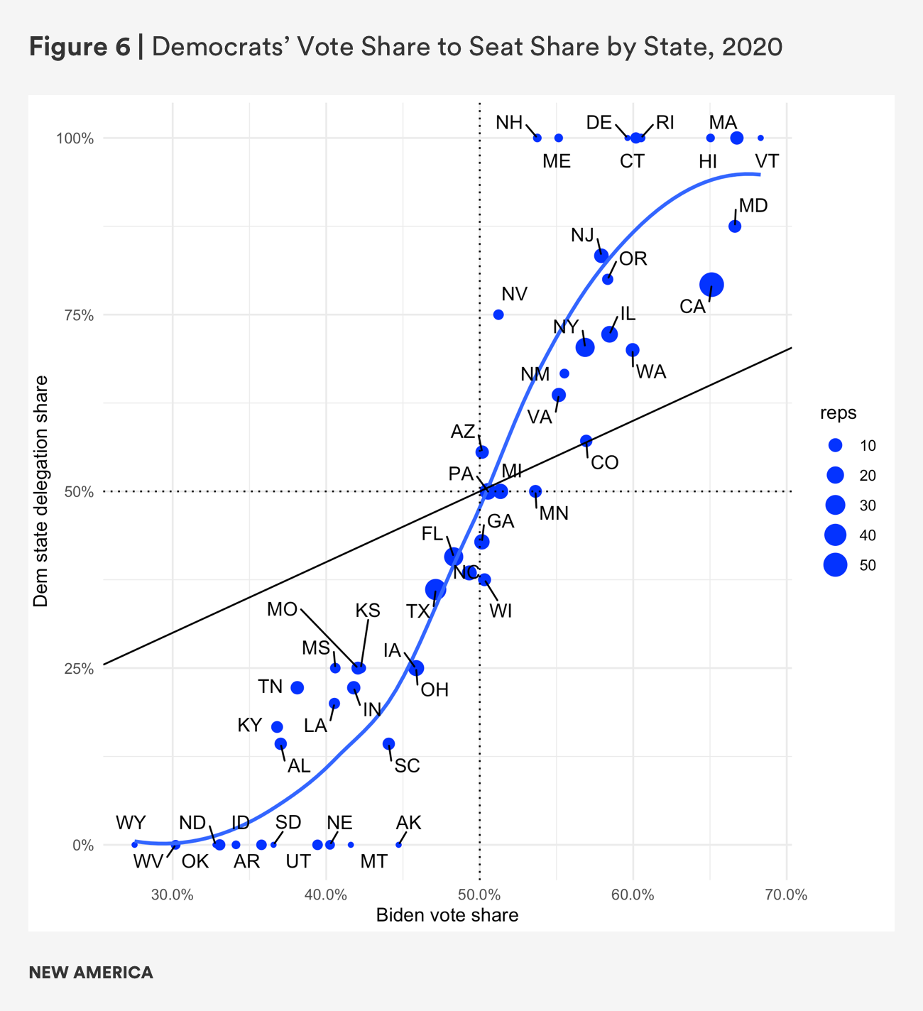
The diagonal line above represents perfect proportionality. Very few states achieve anywhere close to proportionality.

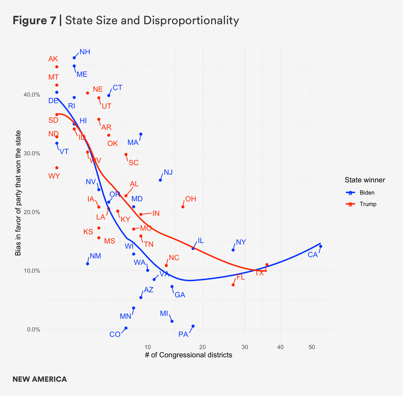
Certainly, as states increase in size, they tend to approach proportionality (zero bias in favor of the party that won the state), but they never achieve it. Notably, Biden states come closer to proportionality on balance than Trump states in the 2020 election.

Symmetry

Acknowledging that perfect proportionality is a chimera in single-member districting, a generation of scholars instead began analyzing districting schemes under the standard of “symmetry.”⁷ That is, if we accept that single-member districts inherently generate a winner’s bonus, then proportionality is not a fair standard. Rather, a fair standard would be that if the vote breaks 52-48 in favor of Democrats, Democrats wind up with the same winner’s bonus that Republicans would wind up with if the vote broke 52-48 towards Republicans.⁸ (And the same if it broke 51-49, or 53-47, etc.)

An even simpler measure, with similar properties, is the mean-median difference. This compares the party’s median vote share minus its mean vote share across all of a plan’s districts. The lower the difference, the more symmetrical (and therefore balanced) the plan. The greater the difference, the higher the level of bias. ⁹

Wasted Votes and “Efficiency” Measures

Another class of partisan fairness measures is built around the concept of “wasted” votes and “efficiency.” Under single-member districts any vote cast in excess of that needed for a majority in a single district, or any vote cast for a losing candidate, is effectively “wasted” or “inefficient.”

Probably the most widely used metric, developed by Eric McGhee and Nick Stephanopolous, is the “efficiency gap” measure.¹⁰ The efficiency gap is the partisan difference between these inefficient votes. If Democrats waste more votes than Republicans, then we can say that the map is biased against Democrats. If Republicans waste more votes, then we can say that the map is biased against Republicans.

The efficiency gap measure gained prominence when plaintiffs utilized it in the Supreme Court partisan gerrymandering cases Whitford v. Gill (2018) and Rucho v. Common Cause (2020). Plaintiffs had hoped that they had finally hit upon a formula to answer Justice Anthony Kennedy’s call in the 2004 Vieth v. Jubelirer decision for a justiciable standard. But in Rucho, the conservative majority declared that partisan gerrymandering was not justiciable; state legislatures could do what they want. Critics of the decision have speculated that perhaps no measure would have been good enough for the conservatives on the Supreme Court. But perhaps it did not help that scholars failed to agree amongst themselves on the proper standard, thus validating the conservatives’ point that any measure would be arbitrary.

A few other measures have built upon the efficiency gap, emphasizing slightly different conceptual baselines of fairness. Rather than taking the absolute difference between wasted votes, some propose taking the difference between the fraction of votes wasted by the party.¹¹

The mathematician Gregory S. Warrington proposes something he calls the “declination,” which measures the “angle associated with the vote distribution.” It is essentially a way of measuring differential responsiveness to vote shifts.¹²

Improbability and Intent

Yet another category of analysis avoids any specific mathematical formula or particular conception of “fairness,” but instead uses computer simulations to demonstrate how unlikely it would be for a given district plan to emerge if line-drawers were acting neutrally. The basic idea here is that intent matters most. Because Democrats naturally over-concentrate their votes in urban areas, it is possible to “unintentionally” draw districts that disadvantage the party.¹³ To differentiate between unintentional/natural partisan gerrymandering and intentional/unnatural partisan gerrymandering, you can ask a computer algorithm to tell you how likely it would be for a given partisan balance to emerge on its own. For example, if a state’s 12 member delegation is eight Republicans and four Democrats, we can ask a computer to draw 10,000 potential maps. Then we can ask how many of those maps generated an 8-4 Republican bias. If the percentage is very low, we can say it is highly improbable that a more neutral process would have generated such a map, and reasonably conclude that the legislature’s intent was.¹⁴

Of course, this approach raises the obvious question: How unlikely should such a map be to declare it as intentionally partisan? And again, there is no perfect standard.

Balance Over the Decade

A final consideration in map-drawing is that maps are drawn with the intention of lasting for a decade—until the next Census. But over the course of a decade, demographics within and across districts may change. And because a portion of the electorate tends to go back and forth between the two parties, or between voting and not voting at all, some years are better years nationwide for Republicans, while other years are better years for Democrats.

The first consideration, the “demographic drift” of a district, means that over the course of a decade, a district drawn to be safe for one party could become competitive. This is referred to as a “dummymander,” and it typically happens when a partisan legislature gets aggressive in drawing an excessive number of seats for its party. ¹⁵ Having a bunch of 55-45 districts can generate an immense partisan advantage in the first election in a decade-long cycle. But if demographics change against your party, those districts will wind up very competitive, erasing the advantage. Similarly (the second consideration), those seats could be vulnerable in a wave election for the opposing party.

Broadly, think of it as a risk-reward tradeoff. A more aggressive partisan gerrymander can leave your party vulnerable in a bad year for your party, because you’ve spread your voters out too diffusely to claim more narrow victories in a good year. A less aggressive partisan gerrymander can preserve seats even as demographics may change, or there may be a wave election against the party. ¹⁶ Broadly, in the latest round of redistricting, Democrats employed the first strategy in the states where they drew the maps, spreading out their voters more efficiently at the risk of losing more seats in an off year. Republicans, by contrast, did more “ring-fencing” in the states where they drew the lines. This means that even in a Democratic year, Democratic gains will be somewhat limited in Republican-controlled states, though Republican gains will also be limited in a Republican year. Or, in terms that we might recognize more clearly, in 2021, Republicans moved more lean Republican seats into solid Republican seats, Democrats moved more solid Democratic seats into lean Democratic seats. We will see how this plays out over the decade.

The Urban-Rural Problem and Single-Member Districts

Obviously, it is highly unlikely that in a two-party system (or really any party system), voters would be equally distributed throughout a state, or throughout a country. Different regions have different cultures. Country life and city life have always had different values and different economies.

Rather, parties are likely to cluster geographically. To some extent, the Republicans and Democrats have always had separate geographical footprints. What is distinct about recent decades, however, is that the sorting of the parties has become much more clearly urban versus rural.

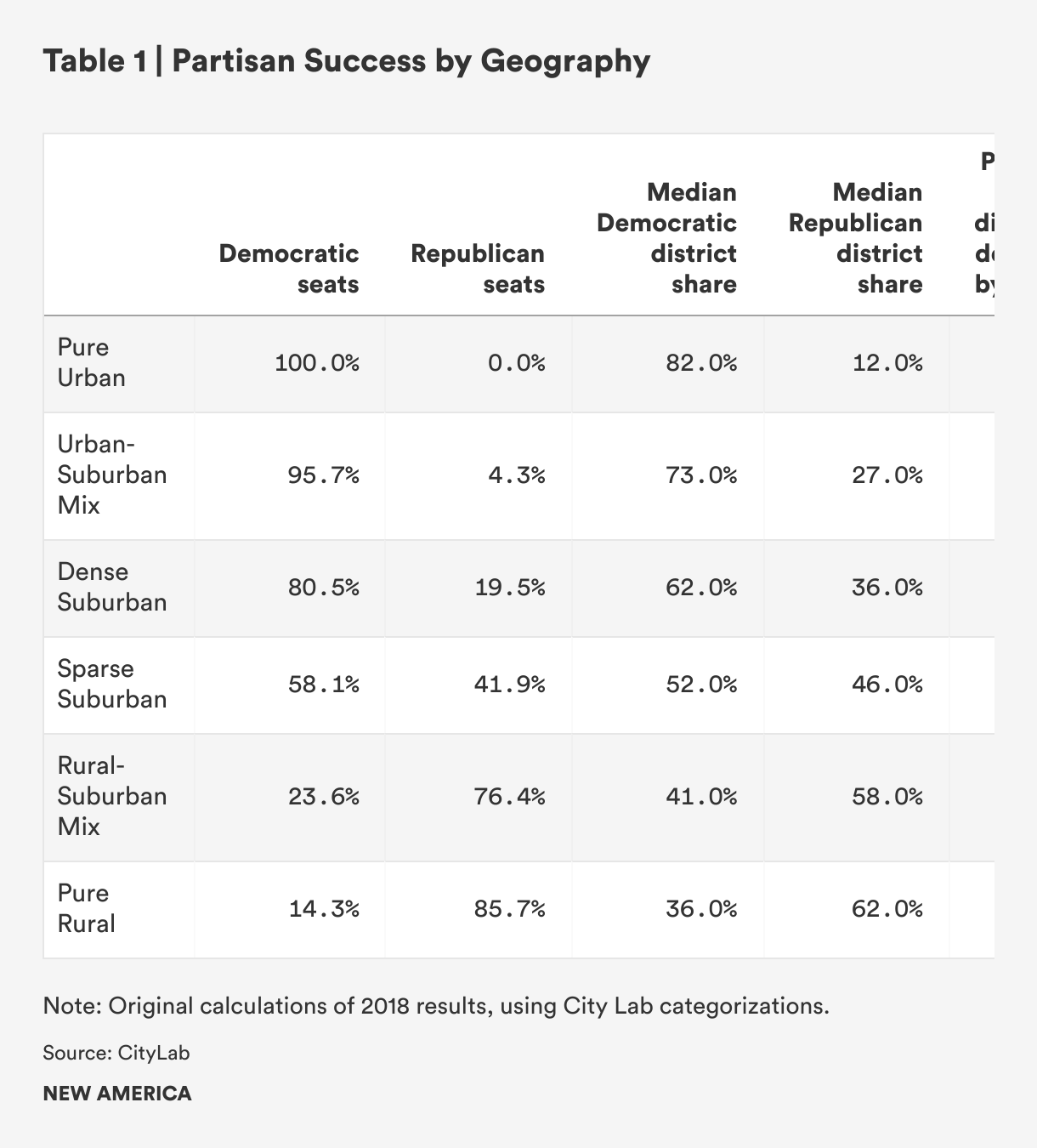
The basic problem for partisan neutrality is that cities are dense population clusters. Since Democrats are the party of the cities, this means that they are likely to live in congressional districts that are extremely Democratic. By contrast, because exurbs and rural areas are much more diffuse, Republican voters wind up being distributed more “efficiently.” That is, they are more likely to live in districts that combine smaller (Democratic) cities and/or suburbs. Many of these districts may be solidly Republican. But they are more likely to be 60 or 65 percent Republican, whereas urban districts are more likely to be 80+ percent Democratic, and the urban-suburban districts are on average 70+ percent Democratic.

This partisan geographic distribution is not unique to the United States. It is a problem for all political systems that use single-member districts. As Jonathan Rodden explains in Why Cities Lose, “Underrepresentation of the urban left in national legislatures and governments has been a basic feature of all industrialized countries that use winner-take-all districts.”¹⁷ This has long been true in the U.K. and Canada, even though both countries use national districting commissions to establish boundaries independently of partisan politics.

Any single-member districting system is going to work against the party that clusters geographically in an “inefficient” manner.¹⁸ This property of single-member districts makes partisan fairness inherently contested. Political scientists sometimes refer to this as “natural gerrymandering”—without any intervention, naturally Democrats “pack” themselves into a smaller number of districts, in effect wasting their votes. Republicans, by contrast, naturally distribute their voters more efficiently by being the exurban party.¹⁹

Partisan Neutrality: The Bottom Line

So what exactly is fair to both parties when it comes to districting? We think we know an extreme gerrymander when we see it. But would we know an extreme map if we saw one? Because single-member districts have several naturally distortive properties, including their high sensitivity to the geographical distribution of voters and the profuse possibilities they afford in drawing boundaries, a unified measure of partisan fairness remains elusive.

It should not be controversial to declare certain partisan maps as extreme partisan gerrymandering. However, as mapmakers approach balance, fairness becomes more sensitive to the metric. Moreover, because some gerrymandering is unintentional (because Democrats concentrate in cities, which creates natural inefficiencies in their distribution) and some is intentional, it is even harder to determine what is fair. Should mapmaking correct for these natural imbalances? Or is that just the fault of Democrats, for doing a poor job of appealing beyond their urban core when they know the consequences of single-member districting?

All of this might not be a problem if American politics were not locked in a high-stakes hyper-partisan doom loop, in which narrow House majorities are up for grabs with each election and the losing side can almost credibly claim that something was unfair about the districting plan if they lost, no matter whether the lines were drawn by a commission or by politicians. This perception of illegitimacy is, of course, a serious problem for our democracy. Commissions may help mitigate the problem slightly, but they certainly cannot eliminate it, given the underlying conditions.

In many respects, competitiveness is the essential quality of electoral democracy. A minimal definition of democracy involves elections with at least two viable parties.²⁰

One well-documented consequence of single-member districts is that even under optimal levels of competitiveness, the majority of districts in any given election are likely to be uncompetitive. Again, this is true in comparable democracies with single-member districts, such as the United Kingdom and Canada. This follows from the realities of partisan geographic clustering. It is almost inevitable that certain parties will be very strong in certain regions of the country, where single-member districts will all but guarantee them a seat.²¹

However, for national elections to be considered competitive, there must be enough competitive districts to hold the balance of national power. But how many?

The potential for competitive districts in a system of single-member elections is really a function of two factors. The first is the share of the electorate that would consider voting for either party in a given election, (i.e., the share of “swing voters”). The second is the geographic dispersion of reliable partisans (i.e., the extent to which partisans are clustered in places with like-minded partisans).

In an electorate in which every voter was a reliable partisan who voted in every election, there would be no competitive elections. But if some share of voters are open to persuasion and if some share of voters may or may not vote based on mobilization, then we can say a district is competitive if these two groups of voters could realistically determine the winner. This combined share, of course, depends on the starting distribution of partisan support. So in a district where the share of Democratic voters outnumber Republicans 65 percent to 35 percent, it would take some rather remarkable persuasion and tremendous mobilization gap to overcome this differential. By contrast, in a 50-50 district, persuasion and mobilization are everything.

The decline of competitive districts in U.S. House elections is a well-described and well-documented story that boils down to two related but distinct trends: the decline in the share of persuadable voters, and the geographical sorting of the parties. The consequence is districts where the balance of persuadable voters is greater than the gap between reliable partisans. This shift has made mobilization even more important, which is one of many factors contributing to increasing levels of hyper-partisan polarization.

Put simply, it is just more difficult today for mapmakers to draw reliably competitive districts, given both the geographical sorting and decline of swing voters.

The Incumbency Factor

In the 1970s, political scientists began to observe a decline in narrowly decided congressional district elections.²² At the time, predictable partisan voting was extremely low, and the share of the electorate willing to consider either party was at a high. However, incumbency reelection rates remained high, because incumbents could use their existing positions to advertise themselves widely in their communities, and bring money back home to the district, bolstering their popularity. They also could use their incumbency to fundraise, and scare off challengers. Voters supported the candidate, not the party.²³

Gerrymandering played a small but sometimes significant role here. In this era of greater bipartisanship, incumbents worked across party lines to keep their districts safe (hence the gerrymandering epithet about politicians picking their voters). At the time, partisan control of Congress was seen as less important to voters. Partially, this was because it was then taken as a given that Democrats had something like a permanent majority in the House (Democrats controlled the House from 1932-1994, with only a few exceptions in the 1950s). Partially, this was because Congress operated in a more bottom-up, committee-oriented way, and so there were many opportunities for Republicans to participate in lawmaking, even if Democrats controlled the majority. Both parties had liberal and conservative wings, and plenty of cross-partisan dealmaking took place. Split-ticket voting was common.

But over the course of a few decades, and especially after a handful of important wave elections (1994, 2006, 2008, 2010), a generation of once-popular incumbents now out of sync with their districts’ partisanship lost their seats (or retired in anticipation of loss.) The number of competitive districts declined over this period. More importantly, the nature of competitive elections changed.

In the past, incumbency offered a significant advantage. Today, the incumbency advantage is marginal, a few points at best, down from about 10 points in the 1970s and 1980s. The nationalization of partisanship has destroyed the incumbent advantage.²⁴ With control of Congress more contested now than ever, and more voters choosing the party (not the candidate), incumbent protection is no longer the driving force motivating gerrymandering.

Congressional and state legislative districts are by nature arbitrary jurisdictions, up for re-evaluation every decade. This is because they are defined not by fixed boundaries, but by population size. Compare them to counties, cities, or towns, whose jurisdictions remain consistent over long periods of time as administrative entities, and often meaningful community identities, even as populations grow (or sometimes shrink). To some extent, neighborhoods or regions also take on distinct identities and are thus meaningful political subdivisions as well.

Districts, by contrast, are defined by population size, which means that the boundaries must change to reflect changing patterns of population. And as population changes within the political subdivisions, mapmakers inevitably have to make tough choices in order to maintain districts of equal size.²⁵

In theory, districts should be meaningful. Various state constitutions and statutes direct mapmakers to keep communities together:²⁶

• Colorado: “Communities of interest, including ethnic, cultural, economic, trade area, geographic, and demographic factors, shall be preserved within a single district wherever possible.”
• Hawaii: “Where practicable, submergence of an area in a larger district wherein substantially different socio- economic interests predominate shall be avoided.”
• Montana: “The commission will consider keeping communities of interest intact. Communities of interest can be Commission based on trade areas, geographic location, communication and transportation networks, media markets, guidelines, Indian reservations, urban and rural interests, social, cultural and economic interests, or occupations and lifestyles.”

Though the sentiment is similar, each state defines the goal of “communities of interest” slightly differently. The basic idea is that districts should represent something meaningful, but with many possible things to represent, there’s often neither a clear prioritization, nor a clear standard of how to measure any of this.²⁷

As the history section discussed, the concept of a “constituency” has always been fraught and complicated in America. Though there is certainly some overlap of geography with the various interests states’ constitutions elevate, not all interests, particularly demographic, economic, and cultural ones, are concentrated enough to form a geographic community of interest. As a geographical unit, the single-member district puts geography as the central property to represent.

Moreover, as districts grow bigger and bigger, it becomes even harder to conceptualize a diverse group of 750,000 (and growing) citizens as a single “constituency.”

Keeping communities of interest together, particularly across redistricting cycles, has a value in ensuring stability of representation. Voters who build a relationship with one member of Congress may find themselves with a new representative after a districting cycle. This can undermine the constituent-representative connection.²⁸

But the trade-off is that sometimes communities need to be split to ensure more competitive districts, since so many communities today are lopsidedly Democratic or lopsidedly Republican.

In a 2011 study, “The Paradox of Redistricting: How Partisan Mapmakers Foster Competition but Disrupt Representation,” Antoine Yoshinaka and Chad Murphy explore the tradeoffs. They conclude: “taken together, our findings lead to an interesting paradox: redistricting can foster electoral competition (which many may find desirable), but it can also sever representational ties between constituents and their representatives (which many may find undesirable).”²⁹

Similarly, in a 2020 study, “Conflicting Goals of Redistricting: Do Districts That Maximize Competition Reckon with Communities of Interest?,” James Gimpel and Lauren Harbridge-Yong tackle this trade-off.³⁰ Their conclusion is simple. It is hard to keep communities of interest together and draw competitive districts. As they write: “the mandates to respect communities of interest while drawing competitive districts are frequently irreconcilable….Because communities of interest often express an enduring and one-sided partisan loyalty, it is difficult to hold them together and also achieve the goal of drawing an evenly balanced district.” (The even partisan division, of course, is necessary to draw competitive districts.)

At one level, this is a mechanical puzzle of assembling equally balanced districts, like tangrams. If political subdivisions (towns, cities, counties, and neighborhoods) represent the building blocks, and these building blocks are overwhelmingly either blue or red, then given the equal population constraints of districting, and the varied sizes of these building blocks, and the requirements that districts at least be somewhat compact, or at the very least contiguous, slotting the variously sized shapes into equal combinations of red and blue is simply impossible in most cases.

But at an even broader level, assembling the blue triangles and the red squares in equal amounts into a single district challenges the idea of the district as a meaningful jurisdiction. If the idea of a district is that it should represent something, then a district that is half red and half blue is more like two separate districts fused together where only half the district can be represented at any given time.

As a result, competitive districts are typically a Republican outer suburb appended to a lopsidedly Democratic inner suburb or college town. As one recent paper describing the failure of competitive districts to lead to moderation explained, “Reformers often idealize such moderate districts because it is believed that they are most conducive to the political competition that is supposed to produce moderate representation. [However], the fact that such districts are more likely to be heterogeneous mitigates their ability to elect moderate legislators.”³¹ In short, purple districts are really split districts, where focusing on base mobilization is a guarantee while trying to court unpredictable and not necessarily moderate swing voters is a gamble.³²

A fourth value in districting is compactness. A more compact district forms a more coherent unit of representation.

But as with the other values, there are competing measures of compactness. Though compactness may appear intuitive at first glance, upon deeper study, scholars have shown that in fact compactness is a complicated multidimensional concept and have offered almost 100 measures of different features of it.” ³³

In general, three main metrics have predominated over the past three decades:

• Roeck scores (which divide the area of the district by the smallest circle that would be able to fully contain the district); ³⁴
• Convex Hull ratios (which divide the area of the district by the smallest convex polygon that would be able to fully contain the district); and
• Polsby-Popper scores (which divide the area of the district by the area of a circle whose perimeter is equal in length to the perimeter of the district).³⁵

As with other criteria, there is no agreement on how to perfectly measure compactness. Neither federal nor state courts have ever struck down a map for not being compact enough, nor have they ever agreed upon a standard. As Keena et al. argue: “identifying violations of compactness often relies upon subjective judgment. It is unlikely that a court will ever endorse a uniform, objective standard for unlawful noncompactness given that the language of compactness laws is often vague.”³⁶

Ultimately, compactness may simply be a “you know it when you see it” kind of thing. It may be in the eye of the beholder. But it also may vary depending on the beholder. Of course, compactness is probably the least important of the criteria. At some level, it may just be a matter of aesthetics. Strange-looking districts are easy fodder for critics of gerrymandering. But sometimes, appearances do matter, and serpentine zig-zags can stand in for wider shenanigans in the drawing of district lines.

A final consideration in fair districting is racial representation. In theory, racial minorities should be represented in the legislature in close proportion to their share in the population. Accurate descriptive representation has significant documented benefits for both minority communities and for the quality of deliberation and ultimately legislation. ³⁷

But how can mapmakers best achieve accurate and diverse representation? For decades, the standard approach has been to draw majority-minority districts (where national racial minorities constitute the majority of voters in the district, increasing the likelihood they will elect a candidate who represents them well). In such districts, Black voters or Hispanic voters form a majority, and therefore are able to elect Black or Hispanic candidates to represent them. These districts have been successful in both elevating minority representatives to Congress and better representing the concerns of minority voters.³⁸

But exactly how to draw such districts today presents some practical questions. One question is what percent of the district needs to be Black or Hispanic in order to elect a Black or Hispanic representative? Or put another way, how likely is it for white voters to support a Black candidate, or a Hispanic candidate? Mapmakers wishing to marginalize minority influence have had the same “cracking or packing” strategies as partisan gerrymandering. They have done so by lowballing the extent to which voting is racially polarized or overstating the extent of racially polarized voting, thus effectively packing minority voters into a few districts.

Indeed, the balance between partisan concerns and minority representation has been a central question in racial redistricting for decades. The key tension is that because minority voters, especially Black voters, are overwhelmingly Democratic, clustering them in safe districts to ensure that they can elect their candidates of choice has added to the “packing” of Democrats into fewer, more lopsided districts, which in turn has helped Republicans. The evidence on this claim was probably stronger in the 1990s, when many of today’s majority-minority districts were first drawn. However, it remains a contested question in the scholarly literature.³⁹

These questions and tensions have been at the center of a key series of Supreme Court cases that have defined questions around racial gerrymandering under Section 2 of the Voting Rights Laws—Thornburg v. Gingles, Shaw v. Reno, Cooper v. Harris, and most recently, Brnovich vs. Democratic National Committee. ⁴⁰

Racial gerrymandering is a highly litigated area, in which the Supreme Court has established tests and criteria for what is and what is not a racial gerrymander. This makes fair minority representation the only area in which the Courts have laid down standards that offer guidance and limitations to mapmakers.

However, most legal experts expect that the Supreme Court is poised to effectively eviscerate the longstanding protections against racial gerrymandering, based on its 2022 decisions to allow maps in Alabama and Louisiana to stand despite challenges that they were racially gerrymandered, and its potentially more radical decision to leave districting entirely up to the state legislatures, a move it has signaled in taking up a North Carolina case, Moore v. Harper.⁴¹

Although there has long been clearer legal criteria around the goal of minority representation than there are for other redistricting goals, these protections have been steadily weakening. Indeed, in the current redistricting cycle, adequate minority representation appears to be stalling in some places, and backsliding in others.⁴²

Indeed as a January 2022 report by the Brennan Center points out, the latest round of Republican maps, especially in the South, have had particularly dire consequences for communities of color.⁴³ As the report explains:

"Predictably, many of this round’s biased maps achieve their skew at the expense of communities of color. Over the past decade, communities of color accounted for nearly all of the country’s population growth. But in redrawing boundaries, Republican map drawers, especially in the South, haven’t just declined to create any new electoral opportunities for these fast-growing communities; in many instances they have dismantled existing districts where communities of color won power or were on the verge of doing so. This brazen attack is unprecedented in scale. In state after state, Republicans are claiming that they are drawing maps on a “race-blind” basis and then defending the resulting racially discriminatory maps on the basis of partisanship, cynically exploiting the loophole left when the Supreme Court declared that federal courts were off-limits to constitutional challenges to partisan gerrymandering. If courts are not willing to carefully probe the intersection of race and politics, the ruse may just succeed.”

Based on where the Supreme Court appears headed, the importance of independent redistricting commissions as protectors of majority-minority districts will become more important, since partisan state legislatures will likely have the freedom to engage in racial gerrymandering, should they so desire.

A second challenge in fair minority representation is the extent to which minority voters live in dense enough clusters to hold influence in a district, without doing injustice to the values of compactness or keeping communities together. Or put another way, the more racial minorities are self-segregated, the easier it is to draw districts where they will wield majority influence. Of course, as segregation has declined in many urban areas over the last several decades (with more people of color moving into the suburbs, and more white people moving into urban cores), the racial self-segregation necessary for majority-minority districts has dissipated.⁴⁴

This dispersion of minority voters makes it more difficult to draw majority-minority districts while maintaining geographic compactness and keeping communities together. It also makes it easier for mapmakers who are not interested in fair representation for minorities to redraw district lines in ways that under-represent minority groups.